Bourbaki (7b): SOTA 7B Algorithms for Putnam Bench (Part I: Reasoning MDPs)

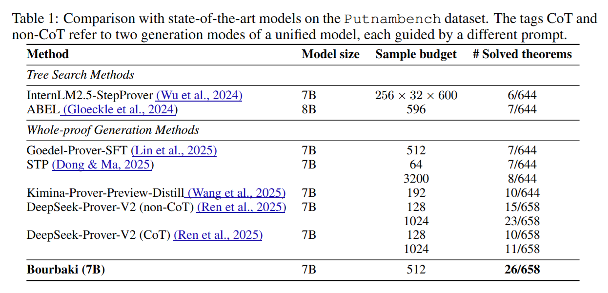
Reasoning remains an open challenge for LLMs. One of the best ways to measure reasoning abilities (from my point of view) is to get LLMs to perform mathematical proofs. When it comes to those, I think PutnamBench is an amazing test - it asks LLMs to prove questions from university level. The authors of PutnamBench have done nothing short of a fascinating job clarifying the importance of such problems and their difficulties. Given their difficulty, it is not surprising that on the leaderboard, the best model (DeepSeek-Proverv2 671B) manages to only prove 47 out of 657 problems in Lean, while the best 7B model (Kimina-Distil) can prove 10. This task is tough!!

In our recent paper, we introduced Bourbaki (7b), an algorithm that operates on top of LLMs to effectively search for proofs in settings where rewards are very sparse. Our search makes use of a variant of Monte-Carlo Tree-Search (MCTS) that we proposed, which approximates the solution to what we called self-generated goal-conditioned MDPs (sG-MDPs). sG-MDPs are a new form of MDPs in which agents generate and pursue their subgoals based on the evolving proof state. Given this more structured generation of goals, the resulting problem becomes more amenable to search. Here, we can apply MCTS-like algorithms to solve the sG-MDP, instantiating our approach in Bourbaki (7b), a modular system that can ensemble multiple 7B LLMs for subgoal generation and tactic synthesis. On PutnamBench, Bourbaki (7b) solves 26 problems, achieving new SOTA results with models at this scale.

Why a Series of Blogs: Well, I want to try to make everyone understand what Bourbaki (7b) is and what it does. I don't want to just give you a ChatGPT summary with some result hype. Bourbaki (7b) is a good start, and I believe it is one of the correct routes we should take when doing proofs. I am hoping with more exposure to this, beyond experiments and codes, some people would be interested and help us improve it! In this first blog, we will be talking basics: 1) MCTS and why it should be applied to LLMs so that the whole world is not just fine-tuning a 100000000000000000000000 b model on 10 data points (not that i have not done it before :-P ), 2) the basics of MDPs, and 3) the Vanilla MCTS algorithm.

Let us Start: Monte Carlo Tree Search (MCTS) is a heuristic method for making optimal decisions. It benefits areas with many choices, such as games, planning and model-based optimisation problems. While the concepts behind MCTS have been around for decades, the method gained significant attention in the mid-2010s due to its success in game-playing AI, e.g., AlphaGo, which used MCTS to beat professional human players in the game of Go. In addition, MCTS has found applications in robotics, automated planning, and even drug discovery. Those successes and the effectiveness of MCTS in handling large search spaces without brute force search made it a valuable tool for modern AI.

In the 2010s and early 2020s, AI graduated from computer games and mastered human-like text generation with the advent of large-scale neural networks, large computing clusters, and internet-scale data. This period saw the rise of large language models (LLMs), which leveraged massive datasets and billions of parameters to achieve unprecedented performance in natural language processing tasks. These models demonstrated a remarkable ability to generate coherent, contextually appropriate text, making them transformative tools that reshaped academia, industry and humanity, I dare to say.

Why MCTS for LLMs: While LLMs excel at producing fluent and contextually relevant responses, they face challenges in tasks requiring long-term planning, reasoning, or exploration of complex decision spaces. This behaviour is unsurprising, given that those models are trained primarily on next-token prediction. Their objective is to generate the next most likely token based on prior context rather than to think ahead strategically or work towards a specific goal. As a result, they could refrain from engaging in goal-conditioned reasoning and instead focus on producing locally plausible outputs that may lack logical consistency. For example, when solving complex mathematical problems or making strategic decisions in a game-like setting, LLMs may generate locally plausible outputs but lack global optimality.

This is one place where Monte Carlo tree search can play a crucial role for LLMs. By integrating MCTS into LLMs' reasoning and decision-making process, it becomes possible to explore multiple potential continuations, simulate their outcomes, and use these simulations to guide the generation process. MCTS provides a potentially practical approach to navigating the vast search space of language generation, balancing the exploration of creative possibilities while exploiting promising paths that meet the goal in question. Incorporating MCTS with LLMs opens up opportunities to:

1. Improve Planning: MCTS can help LLMs evaluate multiple steps ahead, ensuring that decisions align with long-term objectives or constraints;
2. Improve Coherence: By simulating and assessing the outcomes of different branches, MCTS reduces the risk of contradictions or inconsistencies in the generated text;
3. Optimise Reasoning: MCTS allows LLMs to explore diverse problem-solving strategies and identify the most effective approach; and
4. Handle Large Action/Token Spaces: MCTS can systematically explore the vast vocabulary and possible sequences, focusing on the most promising options.

This synergy between MCTS and LLMs holds the potential to address critical limitations in current language models, enabling them to tackle more complex, multi-step reasoning tasks with greater precision and reliability.

Going Back to MDPs:

To better understand how all this would work, let us go back to standard Markov Decision Processes (MDPs) and understand how MCTS is used to solve them. While MCTS can be and has been applied more broadly, in this tutorial, we will solely focus on sequential decision-making problems, which are best formalised as Markov decision processes, or MDPs for short. The following tuple defines an MDP: ℳ = ⟨𝒮, 𝒜, ℛ, 𝒫, γ⟩, such that:

• 𝒮 (States): All possible situations an agent can find itself - e.g., token history for us.
• 𝒜 (Actions): All possible actions the agent can take - e.g., next tokens or steps.
• ℛ (Reward): A function that provides feedback to the agent based on the actions taken - e.g., did we get the correct solution for a math problem?
• 𝒫 (Transition Probabilities): The probabilities of moving from one state to another, given an action - e.g., deterministic in our case (append history with new action).
• γ (Discount Factor): Determines the importance of future rewards - e.g., something like 0.99.

In an MDP, an agent equipped with a policy interacts with the environment over time steps. The policy π: 𝒮 × 𝒜 → [0,1] is an action-selection policy that assigns probabilities for choosing action a in state s. At each time-step, t, the agent observes the current state 𝓈ₜ, selects an action based on its policy 𝒶ₜ ∼ π(⋅|𝓈ₜ), and receives feedback as a reward ℛ(𝓈ₜ,𝒶ₜ). With this, the environment transitions to a new state according to 𝓈ₜ₊₁ ∼ 𝒫(⋅|𝓈ₜ,𝒶ₜ), and the above process repeats. The goal of the agent is to maximise the rewards accumulated along its trajectory:

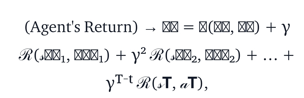
We define the cumulative rewards (returns) at some given time step as follows:

where T is the horizon length or the terminal time step. This equation captures the idea that the agent's decision should not only focus on immediate rewards but also account for future rewards ℛ(𝓈ₜ₊₁, 𝒶ₜ₊₁), ℛ(𝓈ₜ₊₂, 𝒶ₜ₊₂), and so on. The discount factor γ balances the importance of immediate and future rewards since:

• Immediate Rewards: The first term represents the direct feedback the agent receives for its current action. It is weighted higher (with a γ⁰ =1) because it directly reflects the quality of the decision made at time t.
• Future Rewards: The subsequent terms represent the rewards the agent can expect from future decisions. Powers of γ weigh these rewards. This means that rewards further in the future have less impact on the current decision when γ <1 since γ² > γ³ > γ⁴ > …

Of course, our agent's goal is to find the optimal action-selection rule (or policy) which maximises those returns. Before doing so, we first require a measure that evaluates "the goodness" of a state or action under a policy π(⋅|𝓈ₜ). If equipped with this measure, we can optimise for the best policy that maximises it. To quantify this "goodness", we define two functions: the value function, which evaluates the expected return starting from a state, and the Q-function, which assesses the expected return beginning from a state and taking a specific action.

• Value Functions: The value function 𝓥^π(𝓈) = ℰ_{π,𝒫}[𝓖ₜ | 𝓈ₜ = 𝓈], provides a measure of how "good" a state 𝓈 is under a given policy π. It represents the expected cumulative reward the agent can achieve if it starts in the state 𝓈 and follows the policy π after that. This function encapsulates the immediate reward the agent might receive in 𝓈 and the long-term rewards that can be accumulated through future actions guided by π. The value function is beneficial for evaluating the overall desirability of states. If an agent can compare the values of different states, it can prioritise those states that are likely to lead to higher returns in the long run.
• Q-Functions: The Q-function 𝓠^π(𝓈, 𝒶) provides a measure of how "good" it is to take a specific action 𝒶 in a given state 𝓈 under a policy π. It represents the expected cumulative reward the agent can achieve by taking action 𝒶 in state 𝓈 and following the policy π for all subsequent actions. While the value function evaluates the overall desirability of a state, the Q-function extends this evaluation to include specific actions, making it particularly useful for action selection. The agent can determine which actions will lead to higher returns by comparing the Q-values of different actions in the same state. We define 𝓠^π(𝓈, 𝒶) as:
  (Q-Function) → 𝓠^π(𝓈, 𝒶) = ℰ_{π,𝒫}[𝓖ₜ | 𝓈ₜ = 𝓈, 𝒶ₜ = 𝒶].
  Here, the expectation is taken over the trajectory of states and actions induced by π, starting from 𝓈ₜ = 𝓈 and 𝒶ₜ = 𝒶.

The agent must identify the optimal policy to maximise long-term rewards, denoted as π. The optimal policy makes decisions to maximise the expected return in every state. Both the value function 𝓥^π(𝓈) and the Q-function 𝓠^π(𝓈, 𝒶) play a role in defining and finding this optimal policy. More specifically, the optimal policy π can be derived from the optimal Q-function 𝓠^★(𝓈, 𝒶) as follows:

The optimal Q-function 𝓠^★(𝓈, 𝒶) satisfies the following:

This equation simply states that the optimal Q-value for taking action 𝒶 in state 𝓈 is equal to the immediate reward ℛ(𝓈, 𝒶) plus the discounted maximum expected Q-value (i.e., what would we get in the future) of the next state 𝓈'. The discount factor γ determines the importance of future rewards.

While the Q-function evaluates the quality of a specific action in a given state, the overall quality of the state itself, independent of any particular action, is captured by the optimal value function 𝓥^★(𝓈). This function summarizes the maximum expected return achievable from state 𝓈 by choosing the best possible action. Formally, 𝓥^★(𝓈) is defined as:

This equation, known as the Bellman optimality equation for 𝓥^★(𝓈), highlights that the value of a state depends on both the immediate reward ℛ(𝓈, 𝒶) and the expected future rewards, weighted by the transition probabilities and the discount factor γ.

The MCTS Algorithm

Now that we have defined the optimal value function and the optimal Q-function, the next challenge is finding ways to solve MDPs by approximating these terms. While there are multiple approaches to tackle this problem, in this blog, we are primarily interested in planning-based methods, more specifically MCTS. MCTS is particularly effective for planning because it incrementally builds a search tree to approximate the value and Q-functions through simulations. To understand how MCTS operates in the context of MDPs, it is useful to map its components to those of the MDP framework

But What Tree - How to Map MDPs to Search Trees: Before diving into the algorithm searches to find optimal traversal in the tree, we need to understand which tree to construct and how it maps to the MDP we defined above. Let us get started!

1. States as Nodes in the Search Tree: In MCTS, each node in the search tree corresponds to a state 𝓈 ∈ 𝒮 of the MDP. The tree's root node represents the starting state, and the other nodes represent states reachable from the root through sequences of actions. For instance, those nodes also store statistically relevant information that eases the search for optimal policies. Such statistics could, for example, include the number of visits to the current state and cumulative rewards that can be used to estimate Q-values, among others.
2. Actions as Edges Between the Nodes: As we noted earlier, in MDPs, actions 𝒶 ∈ 𝒜 allow the environment to transition from a state 𝓈 to a successor state 𝓈′ according to 𝓈′ ∼ 𝒫(⋅|𝓈, 𝒶). In MCTS, these actions are mapped to edges in the tree. Each edge represents a specific action 𝒶 taken from 𝓈, leading to a new state (or node in the tree) 𝓈′. The tree search will select edges (or actions) based on their estimated Q-values 𝓠(𝓈, 𝒶) stored in the node and visit counts, balancing exploration (attempting less visited states) and exploitation (favouring actions with higher cumulative reward estimates).
3. Rewards and Transitions for Rollouts: MCTS executes simulations or rollouts when searching for optimal policies. During a simulation, the MCTS algorithm samples 𝓈′ based on 𝒫(⋅|𝓈, 𝒶) and accumulates rewards to estimate returns 𝓖ₜ. As such, those rollouts play a critical role in approximating 𝓠(𝓈, 𝒶), where their outcomes are used to update the value estimates stored in the tree nodes.

---

The Vanilla Algorithm: MCTS is an iterative algorithm that incrementally builds a search tree to approximate the optimal value function and the optimal policy. At a high level, it simulates trajectories (rollouts) following the environment's model, collects rewards from the reward function ℛ, and refines the value estimates over time. In detail, the algorithm consists of four main steps: 1) selection, 2) expansion, 3) simulation, and 4) backpropagation.

1) Selection Phase: Starting from the root node (the initial state 𝓈₀), the algorithm traverses the search tree by selecting child nodes (successor states) based on a policy that balances exploration and exploitation. A common selection policy is an adaptation of the upper confidence bound to trees, which we call the upper confidence bound for trees or UCT for short:

where UCT(𝓈, 𝒶) has two terms, one responsible for explotation while the other for exploration that is defined based on visitation statistics:

with β is a parameter trading-off exploration and explotation, N(𝓈) the number of vists to a state 𝓈 and N(𝓈, 𝒶) the number of times an action 𝒶 has been applied in state 𝓈, and ln the natural logarithm.

This UCT formula is designed to handle the exploration-exploitation dilemma, which intuitively boils down to answering the following question: should I rely on what I already know, or should I seek new possibilities?

In our case, if the algorithm only exploits (chooses actions based only on 𝓠(𝓈, 𝒶)), it risks missing better actions that have not been explored enough. On the other hand, if it explores too much, it spends too much time on (potentially) useless actions, harming its convergence to the best strategy. By combining 𝓠(𝓈, 𝒶) with the exploration bonus, UCT can dynamically adjust its behaviour. To understand this, let us examine the equation in more detail and split our analysis into two stages, early and later, during the search.

At the start of the search, the exploration term √(ln [N(𝓈)/N(𝓈, 𝒶)]) dominates because the number of times an action 𝒶 has been taken in state 𝓈, i.e., N(𝓈, 𝒶) is small. This ensures that actions that have been tried less frequently receive a higher exploration bonus, encouraging the algorithm to try them. Note that the numerator grows logarithmically in N(𝓈), ensuring that even as the state 𝓈 is visited many times, the exploration bonus does not grow too quickly. Furthermore, the denominator N(𝓈, 𝒶) is initially very small, boosting the bonus significantly and ensuring that every action gets attempted at least once.

As actions are tried more frequently in the later stages of the search, N(𝓈, 𝒶) grows larger, reducing the exploration term β√(ln [N(𝓈)/N(𝓈, 𝒶)]). At this stage, the Q-value estimate 𝓠(𝓈, 𝒶) term dominates, encouraging the algorithm to favour actions with the highest estimated rewards from past simulations. In other words, it promotes our algorithm to exploit its previous knowledge rather than only exploring. This reflects the algorithm's increasing confidence in its Q-value estimates since the action has been sampled enough times.

2) Expansion Phase: After the selection phase identifies a leaf node (a node which still needs to be fully explored), the algorithm moves to the expansion phase. Expansion aims to grow the search tree by adding one or more child nodes, representing states reachable from the selected leaf node. In other words, the UCT approach described above typically operates on expanded nodes. When it arrives at a leaf node, then expansion begins. This phase incrementally builds the search tree.

During expansion, the algorithm examines the available actions at the selected leaf node. Actions with corresponding child nodes are ignored, as they have already been explored in previous iterations. From the remaining unexplored actions, the algorithm selects one action to expand. This selection is often random or heuristic-based. Once an action is chosen, the algorithm simulates the environment to determine the next state resulting from that action. A new child node is added to the tree, representing this newly reached state. The new child node is initialised with default statistics. Specifically, its visit count N(𝓈') is set to zero. The estimated Q-values for all possible actions at the new node are also set to zero. As more rollouts pass through this node, these values will be updated during the Simulation and Backpropagation phases.

3) Simulation Phase: This is the third step in the MCTS process and is crucial in estimating the value of newly expanded nodes. Once a new node is added to the tree during the Expansion phase, the Simulation phase is used to evaluate the potential of the corresponding state by running a simulated trajectory or rollout from that state to a terminal state (or until a predefined depth). The primary goal of the Simulation phase is to approximate the cumulative reward (or return) obtained starting from the newly added state. During the Simulation phase, the algorithm begins at the newly expanded node, representing a specific state 𝓈. From this state, it simulates a trajectory by repeatedly selecting actions according to a rollout policy. This rollout policy also called the default policy, is typically more straightforward than the UCT-based selection policy used in the tree itself, as the Simulation phase needs to sprint to avoid becoming a computational bottleneck. Common choices for rollout policies include random or heuristic policies. The algorithm selects actions and simulates transitions until reaching a terminal state or a predefined maximum depth. At the end of the simulation, the algorithm computes the trajectory's return 𝓖ₜ.

4) Backpropagation Phase: This final stage of MCTS updates the statistics of the nodes and edges in the search tree based on the results of the Simulation phase. The primary purpose of Backpropagation is to propagate the outcome of the simulated trajectory back up the tree, from the newly expanded node to the root, so that these updates can guide future iterations. Please note that during simulation, we generally do not add new nodes to the tree to avoid a memory explosion. Backpropagation begins at the newly expanded node after computing 𝓖ₜ from a simulation. The cumulative return 𝓖ₜ is passed back up the tree along the path traversed during the Selection phase. At each node along this path, the visit counts N(𝓈), and the action visit counts N(𝓈, 𝒶) are incremented. Furthermore, the Q-value 𝓠(𝓈, 𝒶) is updated to reflect the new information attained from the rollout. Generally, we update those Q-values using the following incremental formula:

For Typos, please comment! I will fix them :-) In the next post, we will detail how we can reframe theorem proving as (goal-conditioned) MDPs, stay tuned!